DBMS: Query Optimization

INTRO 🙌

저번 시간에는 Evaluation of Relational Operations: Other Techniques 에 대하여 알아보았다.

이번 시간에는 Query Optimization에 대해 알아보자.

---

Query Optimization 직관 👀

Plan: RA Tree에서 각 op마다 알맞은 알고리즘 적용 계획

• Each operator typically implemented using a pull interface
  1. OP pulled for the next output \(\rightarrow\) pulls on its inputs
  2. Compute them.
• Two main issues in query optimization★★★★
  • For a given query, what plans are considered?
    • Algorithm to search plan space for cheapest (estimated) plan.
  • How is the cost of a plan estimated?

Ideally: Want to find best plan.

Practically: Avoid worst plans!

We will study the System R approach.

Pipeline vs Batch

Pipeline

• temporary files 활용 빈도 ↓ \(\rightarrow\) the efficiency of the query-evaluation ↑
• faster (= least IO cost); only considering plans that we can pipeline

Batch

• multiple rows at a time
• slower

---

Logical v. Physical Plan 🍞

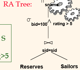
    SELECT  S.sname
    FROM  Reserves R, Sailors S
    WHERE  R.sid=S.sid AND 
        R.bid=100 AND S.rating>5

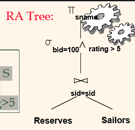
Logical Plan (= RA Tree)

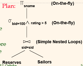
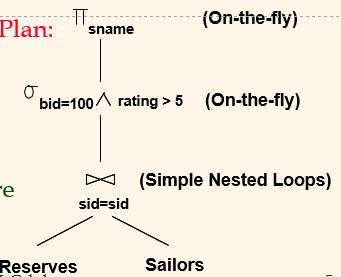
Physical Plan (= Plan)

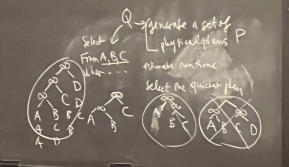
• can be multiple solutions; each can have a different run time

1. generate all possible physical plans
2. estimate the run time of them
3. pick the fastest one.

---

Highlights of System R Optimizer 👌

• 현재 가장 많이 사용됨
• 10개 이하 JOIN에서 잘 동작
• Cost Estimation: Approximate art at best.
  • Statistics (system catalogs) \(\rightarrow\) cost of operations and result sizes.
    • CPU & I/O costs.
• Plan Space: Too large, must be pruned.
  • Only the space of left-deep plans is considered.
    • Left-deep plans allow output of each operator to be pipelined into the next operator without storing it in a temporary relation.
  • Cartesian products avoided.

Best Plan & Cost 계산 ★★★★

예시 1) Two inner-loops (Pipeline)

buffer page 개수 = 2

Outer (Faster)

[\(T\)=outer: faster]

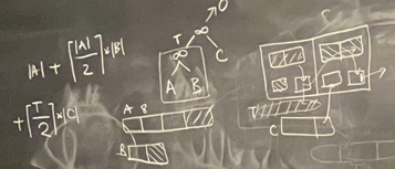
[considered]

Inner (Faster)

[\(T\)=inner: slower]

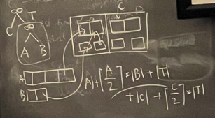
• Pipeline 불가능 \(\rightarrow\) \(\|T\|,\ \|C\|\) 다시 한 번 메모리에 더해주는 모습.

기타

[not considered]

• 3개의 JOIN 연산을 위해 최소한 3개의 메모리 table이 필요한데, 주어진 테이블은 2개이다.

예시 2) Sailors-Reserves

[Relational Schema]

    Sailors (sid: integer, sname: string, rating: integer, age: real)
    Reserves (sid: integer, bid: integer, day: dates, rname: string)

• Reserves: Each tuple is 40 bytes long, 100 tuples per page, 1000 pages.
• Sailors: Each tuple is 50 bytes long, 80 tuples per page, 500 pages.

[RA Tree]

[Query]

    SELECT  S.sname
    FROM  Reserves R, Sailors S
    WHERE  R.sid=S.sid AND 
        R.bid=100 AND S.rating>5

[buffer page 개수 = 5]

상기 relations을 가지고 여러 개의 plans을 만들고 그 cost를 계산해보자.

Plan 1

\[Cost:\ 500+500*1000\ I/Os\]

• 가장 최악 플랜은 아님
• 개선 여지:
  • Selections could have been pushed earlier
  • No use is made of any available indexes
  • etc.

Plan 2 (Pushing Selection)

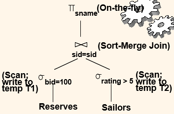
Cost:

• Scan Reserves (1000) + write temp T1 (10 pages, if we have 100 boats, uniform distribution).
• Scan Sailors (500) + write temp T2 (250 pages, if we have 10 ratings).
  • 500 / 2 = 250; 총 10개 ratings 중에 5 이상 선택 –> 나누기 2 (ratings 균등하게 분포되있다고 가정)
• General External Merge Sort
  • Sort T1 (2x2x10), sort T2 (2x4x250), merge (10+250)
  • Total: 4060 I/Os.
    • (1000+500)+(10+250)+(2x2x10+2x4x250+10+250) = 4060
• BNL join
  • join cost = 10+4*250
  • total cost = 2770 I/Os.
    • (1000+500)+(10+4*250)+(250+10) = 2770

General External Merge Sort

pass 개수: \(1+\lceil log_{B-1}(N/B)\rceil\); N=page 개수

Cost: \(2N*(\#\ of\ passes)\).

BNL Join

Cost: \(M+N*\lceil (M/(B-2)) \rceil\).

• If we push projections, T1 has only sid, T2 only sid and sname:
  • T1 fits in 3 pages, cost of BNL drops to under 250 pages, total < 2000.

Plan 3 (Using Indexes: Best)

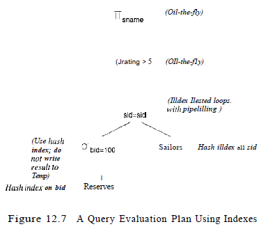
• The selection \(bid = 100\) on Reserves using the hash index \(\rightarrow\) retrieve only matching tuples.

---

Reference

Database Management Systems by Raghu Ramakrishnan and Johannes Gehrke

Relational Operators